Tidymodels
Introduction
RStudio is expanding the tidyverse principles to modelling with R and is building up another metapackage called tidymodels. There are a number of packages at different stages in their development. I am already familiar with rsample and recipes and have tried to implement them in a tidy caret-based modelling workflow before.
- rsample
- recipes
- caret
- 01 robust linear regression,
rlm - 02 neuronal networks,
nnet - 03 multiviariate adaptive regession splines (MARS),
earth
The goal of this post is to check up on all the different packages and try build up a regression modelling workflow using all the appropriate tidymodels tools as soon as they become available at CRAN for I think that this indicates that the authors were confident enough that their package has reached an acceptable stage of maturity.
Packages
CRAN availability of tidymodels packages:
| package | CRAN | description |
|---|---|---|
| broom | Convert statistical analysis objects from R into tidy format | |
| rsample | Classes and functions to create and summarize different types of resampling objects | |
| dials | Tools for creating tuning parameter values | |
| textrecipes | Extra recipes for Text Processing | |
| yardstick | Tidy methods for measuring model performance | |
| parsnip | NR | A tidy unified interface to models |
| probably | NR | Tools for post-processing class probability estimates |
| recipes | A preprocessing engine to generate design matrices | |
| embed | Extra recipes for categorical predictor embeddings | |
| infer | An R package for tidyverse-friendly statistical inference | |
| tidyposterior | Bayesian comparisons of models using resampled statistics |
Unified Modelling Syntax
The declared goal of the tidymodels metapackage is to provide a unified modelling synthax similar to scikit-learn in the python domain or an improved version of caret but adhering to the tidyverse principles. parsnip is going to be the core package while dials will provide suitable objects and functions for parameter tuning. The amount of supported models is still a bit meager so we will not explore these packages any further for the moment.
Statistical Tests and Model Selection
The regular statistical test supported by R have the same problem as the modelling implementations, they lack a uniform tidyverse compatible synthax. Further traditional statistical tests have lately gotten a bit out of fashion. The following criticism keeps popping up:
Specific statistical requirements for each test. The strategies for selecting the right statistical tests are a bit convoluted and a certain set of statistical requirements need to be full-filled for each of them.
Interpretation of P Values. There is a pickiness when it comes to interpreting P Values, the perfect definition eludes me and is completly useless to a none-statistician. Allen Downey has a refreshing practical approach to P values in which he uses a bayesian approach to show that indeed from small p values (<= 0.01) one can conlude that the observed effect has a low probability to be the result of chance (post)
Disregard of Effect Size. If we have a large sample even irrelevant effects will result in low p-values and if we have a small sample only very large effects will result in low p-values. If we detect a relevant effect with a low p-value we cannot be sure that the magnitude of the effect is reproducible. Typically the effect size will decrease the larger the sample. The Null hypothesis does not incorporate a minimum effect size.
As a remedy for the issue of the convoluted statisical requirements for each test a workaround has again been proposed by Allen Downey. He proposes to simulate data that assumes that there is no connection between two hypothetical sets of data that we want to compare (the null hypothesis is true). ( post1, post2 ). Similar to bootstrapping this method is none-parametric and we can use the simulated data to calculate a set of summary statistics. Then we can compare the distribution of these statistics against the actual value. infer allows us to do just that and on-top offers a tidy synthax to the conventional R implementations of standard statistical tests.
However even the simulation technique does not really help us to judge the effect size properly. This is something that can be adressed using bayesian modelling techniques, which will provide you with a posterior distribution of your response variable which allows you to sufficiently judge the effect size.
When using any k-fold cross-validation strategy for model training and validation we can apply statistical tests on each set of k performance metrics to select the best performing model. In general we run into the same issues as discussed above. In order to adress them we can either use the simulation technique of the inferpackage or use tidyposterior which uses Bayesian modelling to compare performance metrics which allows us to define a relevant effect size to test against.
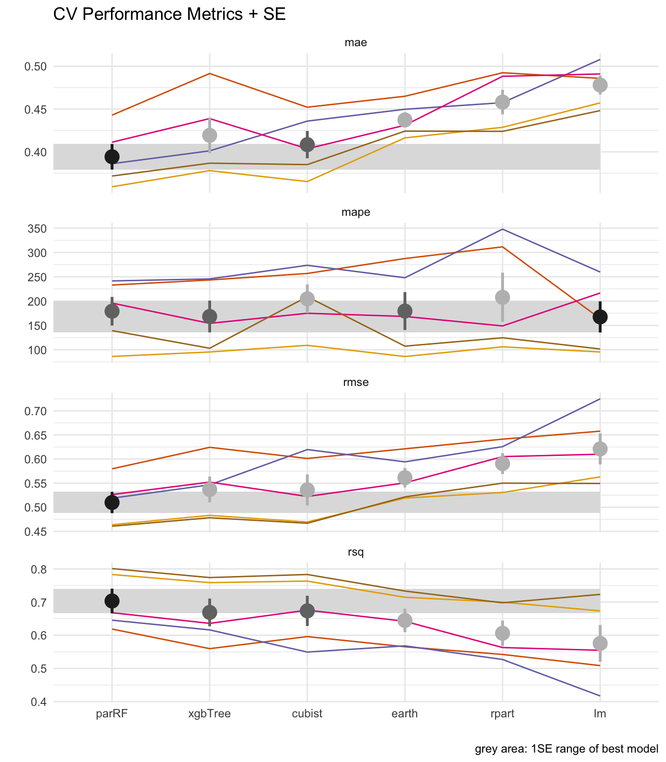
In general I think tidyposterior is probably best practise, however to reduce complexity I am personally quite happy with the 1 SE rule. Simply plotting the mean value with the SE and then picking the simplest model that is within 1SE of the model with the highest performance. Thus I will not include these packages in my modelling workflow for the moment.
Resampling, Feature Engineering and Performance Metrics
rsample, recipes and yardstick are packages that give an overall complete impression and can be used with caret. rsample allows us to create cross validation pairs by indexing an existing dataframe and facilitates the use of modelling dataframes. If supports a variety of resampling methods such as not only limited to k-fold cross validation but also bootstrapping and nested cross validation. recipes allows straight forward feature engineering and preprocessing and yardstick allows us to easily calculate performance metrics from model predictions.
Modeling
We will fit the following regression models to the Boston Housing Data Set
- xgbTree
- lm
- randomForest
- MARS
- Cubist
- CART tree
For tuning we will use a randomized parameter search in a 5-fold cross validation
We will use the following packages:
-recipes
-resample
-caret
-yardstick
-easyalluvial (for color palette)
suppressPackageStartupMessages( library('mlbench') )
suppressPackageStartupMessages( library('tidyverse') )
suppressPackageStartupMessages( library('recipes') )
suppressPackageStartupMessages( library('caret') )
suppressPackageStartupMessages( library('Hmisc') )
suppressPackageStartupMessages( library('xgboost') )


# ggplot default theme
theme_set(theme_minimal())

# Register mutiple cores for parallel processing
suppressPackageStartupMessages( library(parallel) )
suppressPackageStartupMessages( library(doParallel) )
cluster <- makeCluster(detectCores() - 1) ## convention to leave 1 core for OS
registerDoParallel(cluster)
```
Data
data('BostonHousing')
df = as_tibble( BostonHousing )
summary(df)
## crim zn indus chas nox
## Min. : 0.00632 Min. : 0.00 Min. : 0.46 0:471 Min. :0.3850
## 1st Qu.: 0.08205 1st Qu.: 0.00 1st Qu.: 5.19 1: 35 1st Qu.:0.4490
## Median : 0.25651 Median : 0.00 Median : 9.69 Median :0.5380
## Mean : 3.61352 Mean : 11.36 Mean :11.14 Mean :0.5547
## 3rd Qu.: 3.67708 3rd Qu.: 12.50 3rd Qu.:18.10 3rd Qu.:0.6240
## Max. :88.97620 Max. :100.00 Max. :27.74 Max. :0.8710
## rm age dis rad
## Min. :3.561 Min. : 2.90 Min. : 1.130 Min. : 1.000
## 1st Qu.:5.886 1st Qu.: 45.02 1st Qu.: 2.100 1st Qu.: 4.000
## Median :6.208 Median : 77.50 Median : 3.207 Median : 5.000
## Mean :6.285 Mean : 68.57 Mean : 3.795 Mean : 9.549
## 3rd Qu.:6.623 3rd Qu.: 94.08 3rd Qu.: 5.188 3rd Qu.:24.000
## Max. :8.780 Max. :100.00 Max. :12.127 Max. :24.000
## tax ptratio b lstat
## Min. :187.0 Min. :12.60 Min. : 0.32 Min. : 1.73
## 1st Qu.:279.0 1st Qu.:17.40 1st Qu.:375.38 1st Qu.: 6.95
## Median :330.0 Median :19.05 Median :391.44 Median :11.36
## Mean :408.2 Mean :18.46 Mean :356.67 Mean :12.65
## 3rd Qu.:666.0 3rd Qu.:20.20 3rd Qu.:396.23 3rd Qu.:16.95
## Max. :711.0 Max. :22.00 Max. :396.90 Max. :37.97
## medv
## Min. : 5.00
## 1st Qu.:17.02
## Median :21.20
## Mean :22.53
## 3rd Qu.:25.00
## Max. :50.00Response Variable lstat
p_hist = ggplot(df) +
  geom_histogram( aes(lstat) ) +
  lims( x = c(0,40) )

p_ecdf = ggplot(df) +
  stat_ecdf(aes(lstat) ) +
  lims( x = c(0,40) )

gridExtra::grid.arrange( p_hist, p_ecdf )
## `stat_bin()` using `bins = 30`. Pick better value with `binwidth`.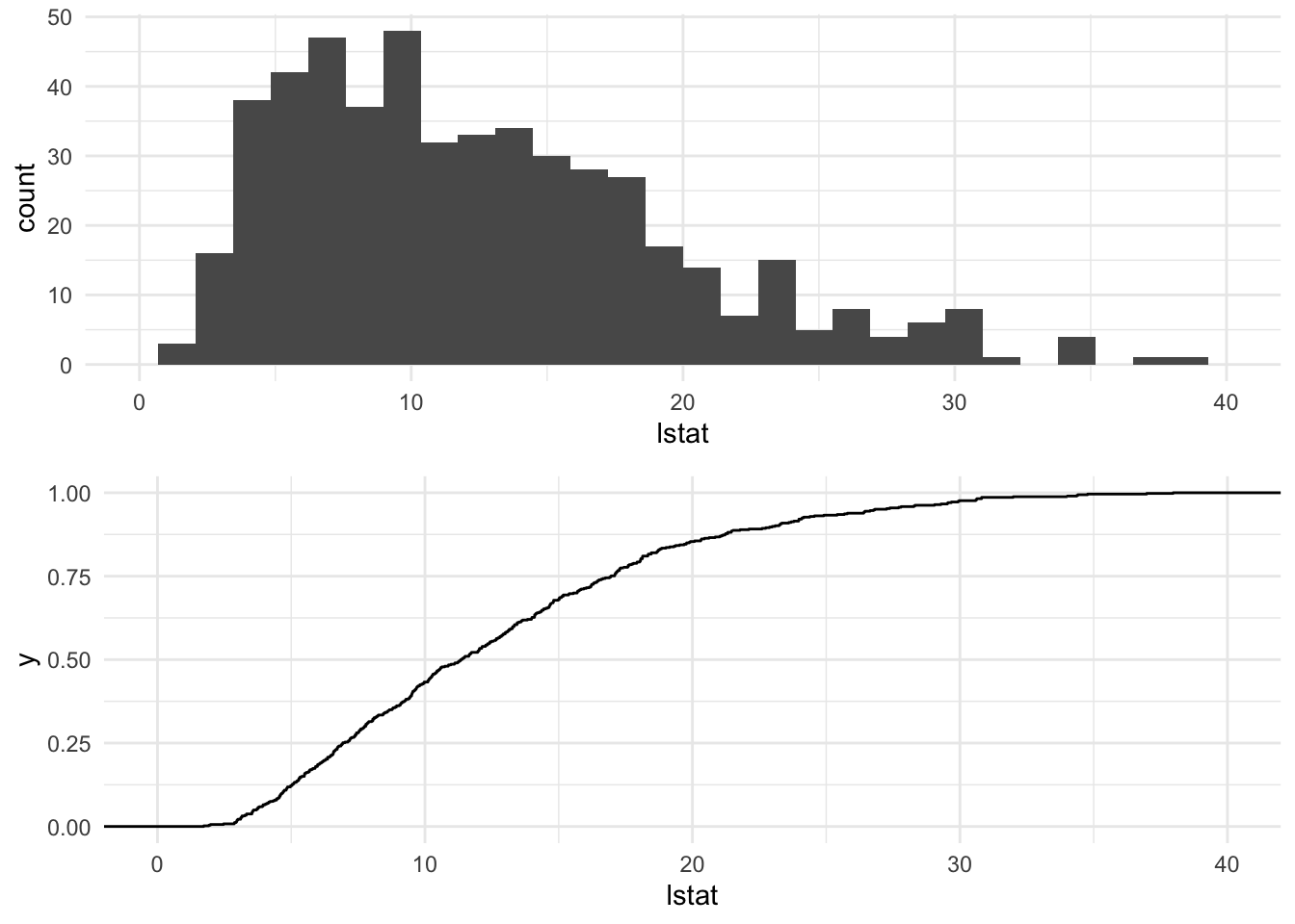
Correlations
df_cor = df %>%
  select_if( is.numeric ) %>%
  gather( key = 'variable', value = 'value', - lstat) %>%
  group_by(variable) %>%
  nest() %>%
  mutate( cor = map_dbl(data, function(x) cor(x$lstat, x$value) ) ) %>%
  unnest(cols = c(data)) %>%
  ungroup() %>%
  mutate( variable = fct_reorder(variable, cor)
          , cor = round(cor,2) )

df_label = df_cor %>%
  group_by( variable, cor) %>%
  summarise( pos = max(value) *.9 )

ggplot( df_cor, aes(lstat, value) ) +
  geom_point( alpha = 0.2 ) +
  geom_smooth( method = 'lm') +
  geom_label( aes( x = 5, y = pos, label = cor)
             , df_label
             , color = 'pink') +
  facet_wrap(~variable, scales = 'free_y')
## `geom_smooth()` using formula 'y ~ x'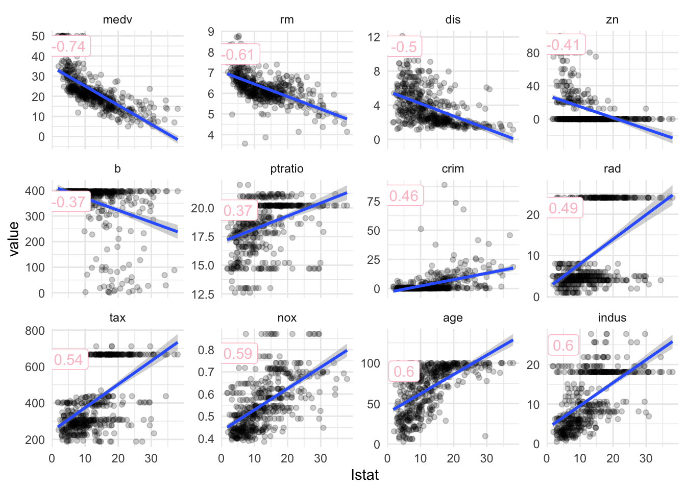
lstat vs categorical variables
df %>%
  select_if( is.factor ) %>%
  bind_cols( df['lstat'] ) %>%
  gather( key = 'variable', value = 'value', - lstat) %>%
  ggplot( aes( x = value, y = lstat) ) +
  geom_violin() +
  geom_boxplot( alpha = 0.5 ) +
  ggpubr::stat_compare_means() +
  facet_wrap( ~ variable )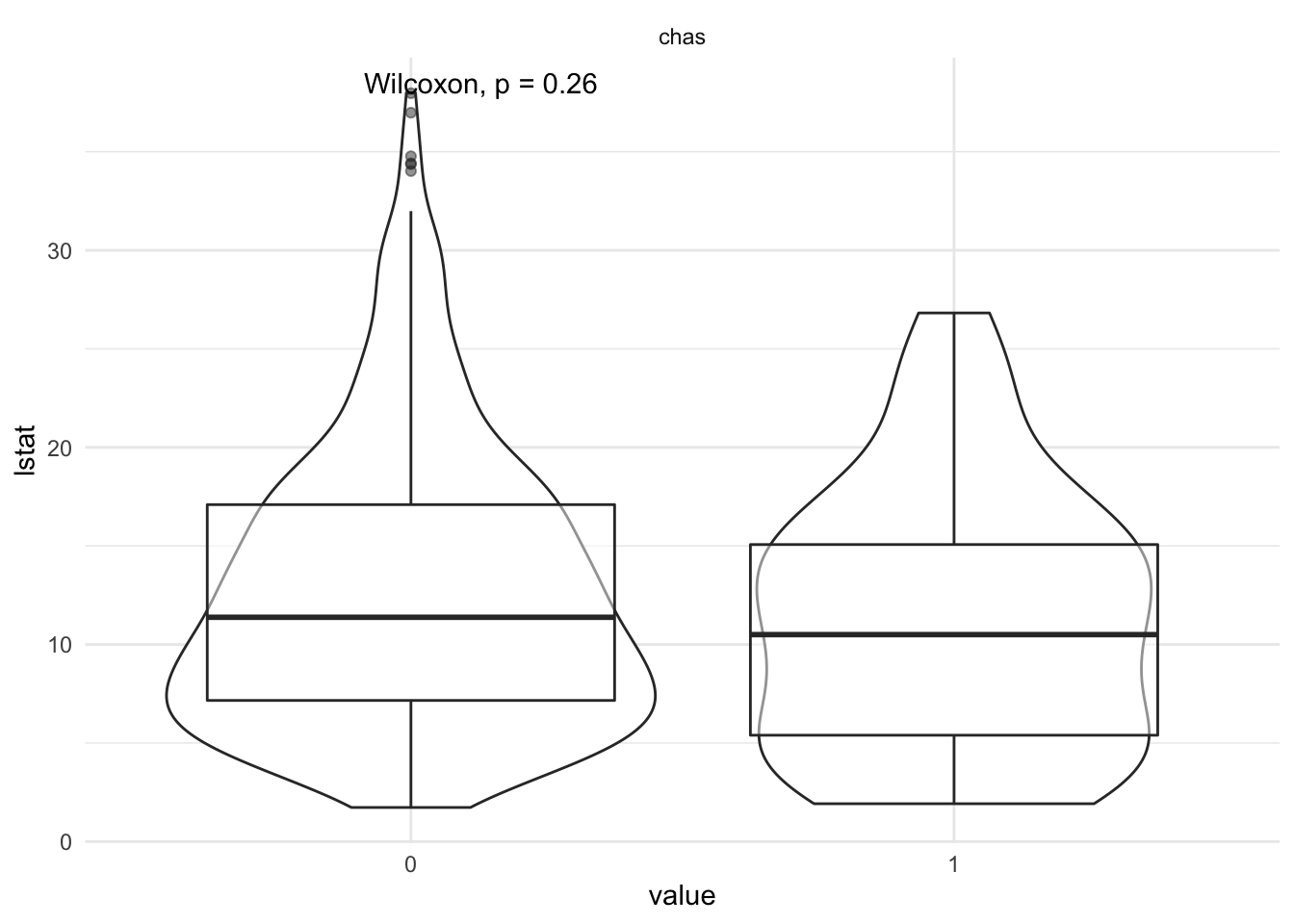
Preprocessing with recipe

Note we are intentionally standardizing the response variable since the unit of lstat is irrelevant for this demo
We will
- Yeo Johnson Transform
- Scale
- Center
- remove co-correlating variables (threshold 0.5)
- dummy encode
rec = recipe(df, lstat ~ . )

summary(rec)
## # A tibble: 14 x 4
## variable type role source
## <chr> <chr> <chr> <chr>
## 1 crim numeric predictor original
## 2 zn numeric predictor original
## 3 indus numeric predictor original
## 4 chas nominal predictor original
## 5 nox numeric predictor original
## 6 rm numeric predictor original
## 7 age numeric predictor original
## 8 dis numeric predictor original
## 9 rad numeric predictor original
## 10 tax numeric predictor original
## 11 ptratio numeric predictor original
## 12 b numeric predictor original
## 13 medv numeric predictor original
## 14 lstat numeric outcome originalrec = rec %>%
step_scale( all_numeric() ) %>%
step_center( all_numeric() ) %>%
step_YeoJohnson( all_numeric() ) %>%
step_corr( all_numeric(), - all_outcomes(), threshold = 0.5 ) %>%
step_dummy( all_nominal() )Summary Recipe
prep_rec = prep(rec, df)
prep_rec
## Data Recipe
##
## Inputs:
##
## role #variables
## outcome 1
## predictor 13
##
## Training data contained 506 data points and no missing data.
##
## Operations:
##
## Scaling for crim, zn, indus, nox, rm, age, dis, rad, ... [trained]
## Centering for crim, zn, indus, nox, rm, age, dis, rad, ... [trained]
## Yeo-Johnson transformation on crim, zn, indus, nox, rm, age, ... [trained]
## Correlation filter removed indus, nox, age, dis, tax, medv, crim [trained]
## Dummy variables from chas [trained]df_prep = bake(prep_rec, df )Resampling with rsample

rs = rsample::vfold_cv(df, v = 5)

rsample::pretty.vfold_cv(rs)
## [1] "5-fold cross-validation"Convert to caret-compatible object
rs_caret = rsample::rsample2caret(rs)Modelling with caret
Wrapper
We will be using randomized parameter search instead of grid search despite the author’s suggestions. It is purely for convenience since it will automatically pick parameters within a sensible range for each model. If we would not automate that we would have to look up the ranges in the documentation or determine them empirically.
car = function( method, recipe, rsample, data){


  car = caret::train( recipe
                      , data
                      , method = method
                      , trControl = caret::trainControl(index = rsample$index
                                                        , indexOut = rsample$indexOut
                                                        , method = 'cv'
                                                        , verboseIter = T
                                                        , savePredictions = T
                                                        , search = 'random')
                      , metric = 'RMSE'
                      , tuneLength = 100
                       )

  return( car )
}

# c = car( 'lm', rec, rs_caret, df)
Apply Wrapper
df_m = tibble( methods = c('lm', 'rpart', 'cubist', 'parRF', 'earth', 'xgbTree') )df_m = df_m %>%
mutate( c = map(methods, car, rec, rs_caret, df ) )Assess Performance with yardstick

df_pred = df_m %>%
  mutate( pred = map(c, 'pred' )
          , pred = map(pred, as_tibble )
          , best_tune = map(c, 'bestTune') )

df_pred
## # A tibble: 6 x 4
## methods c pred best_tune
## <chr> <list> <list> <list>
## 1 lm <tran.rcp> <tibble [506 × 5]> <df[,1] [1 × 1]>
## 2 rpart <tran.rcp> <tibble [18,216 × 5]> <df[,1] [1 × 1]>
## 3 cubist <tran.rcp> <tibble [48,070 × 6]> <df[,2] [1 × 2]>
## 4 parRF <tran.rcp> <tibble [3,036 × 5]> <df[,1] [1 × 1]>
## 5 earth <tran.rcp> <tibble [13,156 × 6]> <df[,2] [1 × 2]>
## 6 xgbTree <tran.rcp> <tibble [50,600 × 11]> <df[,7] [1 × 7]>filter(df_pred, methods == 'cubist') %>%
.$pred ## [[1]]
## # A tibble: 48,070 x 6
## obs rowIndex pred committees neighbors Resample
## <dbl> <int> <dbl> <int> <int> <chr>
## 1 -1.87 4 -1.32 3 5 Fold1
## 2 0.740 8 -0.0712 3 5 Fold1
## 3 1.55 9 0.616 3 5 Fold1
## 4 0.855 11 -0.240 3 5 Fold1
## 5 -0.351 15 -0.0309 3 5 Fold1
## 6 -0.123 19 1.15 3 5 Fold1
## 7 0.481 26 1.06 3 5 Fold1
## 8 0.292 27 0.225 3 5 Fold1
## 9 0.560 28 0.608 3 5 Fold1
## 10 -0.0793 30 -0.0862 3 5 Fold1
## # … with 48,060 more rowsParameters as string
We need to horizontally concat all parameter columns into two columns that are the same for all models otherwise we will not be able to unnest the predictions. We need to convert strings to symbols in order to use them for dplyr functions (see programming with dplyr ).
params_as_str = function(df, params){

  symbols = map( names(params), as.name )

  df %>%
    mutate( desc_values = pmap_chr( list( !!! symbols), paste )
            , desc_params = paste( names(params), collapse = ' ' ) )
}

# params_as_str(df_pred$pred[[6]], df_pred$best_tune[[6]] )
Apply and unnest
df_pred = df_pred %>%
  mutate( pred = map2(pred, best_tune, params_as_str )
          , pred = map(pred, select, Resample, desc_params, desc_values, rowIndex, obs, pred)
          ) %>%
  unnest(pred)

df_pred
## # A tibble: 133,584 x 9
## methods c Resample desc_params desc_values rowIndex obs pred
## <chr> <lis> <chr> <chr> <chr> <int> <dbl> <dbl>
## 1 lm <tra… Fold1 intercept TRUE 4 -1.87 -0.815
## 2 lm <tra… Fold1 intercept TRUE 8 0.740 -0.627
## 3 lm <tra… Fold1 intercept TRUE 9 1.55 -0.177
## 4 lm <tra… Fold1 intercept TRUE 11 0.855 -0.726
## 5 lm <tra… Fold1 intercept TRUE 15 -0.351 0.0395
## 6 lm <tra… Fold1 intercept TRUE 19 -0.123 0.644
## 7 lm <tra… Fold1 intercept TRUE 26 0.481 0.534
## 8 lm <tra… Fold1 intercept TRUE 27 0.292 0.250
## 9 lm <tra… Fold1 intercept TRUE 28 0.560 0.218
## 10 lm <tra… Fold1 intercept TRUE 30 -0.0793 -0.331
## # … with 133,574 more rows, and 1 more variable: best_tune <list>Get best performing model for each method
df_best_models = df_pred %>%
  group_by( methods, desc_params, desc_values) %>%
  yardstick::rmse(obs, pred) %>%
  group_by( methods ) %>%
  mutate( rnk = rank(.estimate, ties.method = 'first' ) ) %>%
  filter( rnk == 1 ) %>%
  select( - rnk ) %>%
  arrange(.estimate) %>%
  ungroup() %>%
  mutate( methods = fct_reorder(methods, .estimate) )

df_best_models
## # A tibble: 6 x 6
## methods desc_params desc_values .metric .estimator .estimate
## <fct> <chr> <chr> <chr> <chr> <dbl>
## 1 parRF mtry 2 rmse standard 0.512
## 2 xgbTree nrounds max_depth e… 638 4 0.02251800388… rmse standard 0.540
## 3 cubist committees neighbors 36 8 rmse standard 0.540
## 4 earth nprune degree 8 2 rmse standard 0.563
## 5 rpart cp 0.00450606062062921 rmse standard 0.592
## 6 lm intercept TRUE rmse standard 0.624Get cv-performance
performance = yardstick::metric_set( yardstick::rmse, yardstick::rsq, yardstick::mae, yardstick::mape )

df_perf = df_best_models %>%
  select(methods, desc_params, desc_values) %>%
  left_join(df_pred) %>%
  group_by( methods, Resample) %>%
  performance(obs, pred) %>%
  mutate( methods = as.factor(methods)
          , methods = fct_relevel(methods, levels(df_best_models$methods) )) %>%
  group_by(methods, .metric) %>%
  mutate( me = mean(.estimate)
             , se = sd(.estimate)/sqrt(n()) )
## Joining, by = c("methods", "desc_params", "desc_values")Get 1SE stats
df_1se = df_perf %>%
  group_by(methods, .metric, me, se) %>%
  summarise() %>%
  mutate(  ymin = me - se
          , ymax = me + se ) %>%
  group_by(.metric) %>%
  mutate( rnk = rank(me, ties.method = 'first')
          , rnk_desc = rank( desc(me), ties.method = 'first')
          ) %>%
  rename( best_method = methods ) %>%
  filter( (rnk == 1 & .metric != 'rsq') | (.metric == 'rsq' & rnk_desc == 1) )

df_1se
## # A tibble: 4 x 8
## # Groups: .metric [4]
## best_method .metric me se ymin ymax rnk rnk_desc
## <fct> <chr> <dbl> <dbl> <dbl> <dbl> <int> <int>
## 1 parRF mae 0.394 0.0149 0.379 0.409 1 6
## 2 parRF rmse 0.510 0.0221 0.488 0.532 1 6
## 3 parRF rsq 0.703 0.0372 0.666 0.740 6 1
## 4 lm mape 167. 32.0 135. 199. 1 6Plot
len = levels(df_perf$methods) %>%
  length()

col_class = RColorBrewer::brewer.pal('Greys', n = 9) %>% rev()
col_folds = RColorBrewer::brewer.pal('Dark2', n = 8) %>%
  easyalluvial::palette_filter(greens = F, greys = F)

pal = c( col_class[2], col_folds[1:5], col_class[4], col_class[6] )

df_perf %>%
  left_join( select(df_1se, .metric, ymin, ymax, best_method) ) %>%
  mutate( classification = case_when( best_method == methods ~ 'best'
                                      , me >= ymin & me <= ymax ~ 'in'
                                      , T ~ 'out' )
          ) %>%
  ggplot( aes(methods, .estimate) ) +
    geom_rect( aes(ymin = ymin, ymax = ymax )
               , xmin = 0, xmax = len
               , fill = col_class[7]
               , alpha = 0.05 ) +
    geom_line( aes( group = Resample, color = Resample)
               , size = .5, alpha = 1 ) +
    stat_summary( aes( color = classification)
                  , size = 1
                  , fun.data = function(x) mean_se( x, mult = 1) ) +
    scale_color_manual( values = pal ) +
    theme( legend.position = 'none') +
    labs( y = '', x = '', caption = 'grey area: 1SE range of best model'
        , title = 'CV Performance Metrics + SE') +
    facet_wrap(~.metric, scales = 'free_y', ncol = 1)
## Joining, by = ".metric"